
In-process gauging of bearing balls: nanometric measurement with Python in 10 minutes
A manufacturer of spherical rolling elements, bearing balls and rollers, produces at high volume against tight dimensional tolerances. Diameter and length are checked after the part leaves the process, on a sampling basis. Every out-of-tolerance part found at that point has already been mixed with good parts, already moved downstream, and sometimes already shipped. Scrap is discovered late, rework is expensive, and a customer complaint costs more than either.
1. Challenge
Gauging a part while it moves is a different problem from gauging it on a bench.
The tolerance is the first constraint: on a precision rolling element, the differences that matter sit well below the micrometre, so the measurement chain has to resolve dimensional change at a scale where cable noise, temperature drift and a slow ADC all become the dominant error. The second constraint is timing, the part is in the measurement zone briefly, and there is no dwell time in which to take a careful reading. The third is architecture: several probes must be acquired together and attributed to the same part as it passes, then reduced to a single pass/fail number fast enough for the PLC to act on it in the same cycle.
Most integrations solve this by adding hardware, a presence sensor to say when the part is there, a PC to do the maths, a conditioning rack between probes and acquisition. Each addition is another item to wire, align, power and maintain, and another place for the measurement to go wrong.
2. Solution
Put the acquisition on the machine, and let it do the reduction itself.
Die ADDI-DATA MSX-E3701 is a rugged IP 65 metal-housed Ethernet system (−40 to +85 °C) that drives 8 or 16 inductive displacement transducers directly (Half-Bridge, LVDT, Mahr-compatible or Knaebel) with no external conditioner. It generates the transducer supply itself (differential sine, 5 to 50 kHz) and digitises at 24-bit.
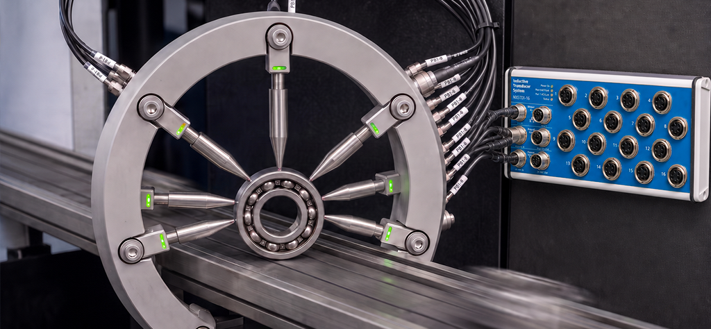
In this application six probes are mounted as three facing pairs on a ring the part is pulled through. The module runs a peak-hold (min/max) acquisition: it tracks the extremum on every channel in hardware while the part passes, and this is the part that removes components from the bill of materials, it can stop itself on a threshold crossing. When a watched probe falls back past a configured value, the part has cleared, and the acquisition ends. No presence sensor. No polling loop deciding when the part arrived.
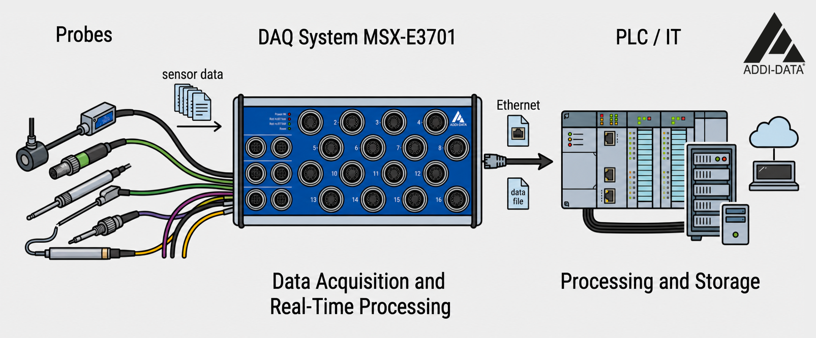
Where does it fit in your architecture? Your probes stay yours. Your PLC and your IT stack stay yours, unchanged. The MSX-E3701 owns the level in between acquisition – reduction, and hands over a result that is already a measurement, not a raw signal.
Accuracy: what the numbers actually mean
The measurement range is not fixed by the module. It is set by the transducer fitted and selected in software, which is why the same hardware serves a micrometric gauging job and a millimetre-range positioning job.
Accuracy is 16-bit over whatever range you choose. The datasheet’s worked example: a TESA GT21 with a ±2 mm range (Δ 4 mm) gives 4 mm ÷ 2¹⁶ = ±61 nm, or 0.061 µm. Fit a narrower-range probe and the same 16 bits resolve proportionally finer. That relationship accuracy scales with the range you select is the whole reason tight-tolerance in-process gauging is viable on a general-purpose platform.
Key features
- 8 or 16 inputs for inductive transducers, 24-bit, 5-pin M18 female connectors
- Half-Bridge, LVDT, Mahr-compatible or Knaebel, no external signal conditioner
- On-board sine wave generator for transducer supply (5 / 7.69 / 10 / 12.5 / 20 / 50 kHz)
- Peak-hold (min/max) acquisition computed on the module, with self-stop on threshold
- Transducer diagnosis: line break and short-circuit detection, per channel
- On-board transducer database and guided calibration
- 24 V hardware trigger in/out; µs-level synchronisation between cascaded systems
- ARM®9 32-bit processor, robust standardised metal housing, IP 65
- 1000 V optical isolation, ±40 V overvoltage protection, 150 m cable on CAT5E
3. Ten-Minute Quick Start
Step 1: Configure MSX-E
Connect the MSX-E3701 to your Ethernet network. The module ships with a default IP address; set it to match your network with ADDI-DATA ConfigTools (included in delivery).
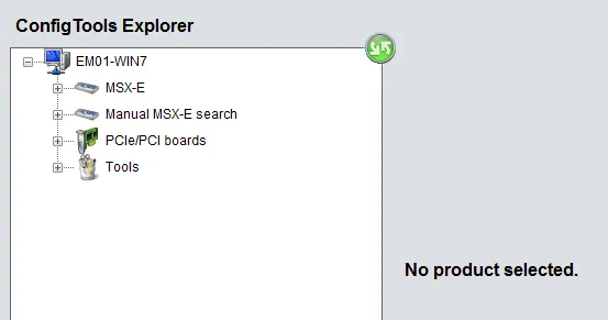
Übersicht ConfigTools-Fenster
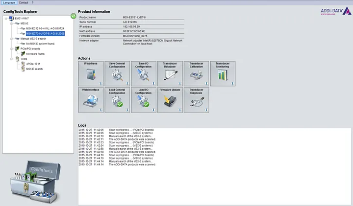
Step 2: Install the API
Clone the open-source samples from github.com/ADDI-DATA/msxe-samples and install the runtime dependencies:
pip install zeep numpyThe WSDL service definitions are bundled with the API. The client starts fully offline, no internet access and no proxy configuration.
Step 3: Ask the module what it can measure with
Before anything else, find out which transducer types this module knows and what range each one covers. The selection_index printed here is the value every acquisition call needs.
from msxe_api import MSXE370xAPI
from msxe_api.msxe370x import TYPE_NAMES

msxe = MSXE370xAPI("192.168.99.99")          # SOAP control on :5555

for index in range(msxe.get_number_of_types()):
    info = msxe.get_type_information(index)
    print(f"[{info['selection_index']}] {info['name']} "
          f"({TYPE_NAMES.get(info['type'])})")
    print(f"    range       : {info['range_mm']} mm")
    print(f"    sensitivity : {info['sensitivity_mv_v_mm']} mV/V/mm")
    print(f"    frequency   : {info['frequency_hz']} Hz")
Reading the range from the device rather than hardcoding it matters: a fixed constant silently produces wrong millimetre values the day someone fits a different probe.
Step 4: First peak-hold measurement
This is the classic gauging pattern. Start a min/max acquisition, let the part pass, read the extremum per channel. No data travels to the data server in this mode, the values come back from the status call.
import time
from msxe_api import MSXE370xAPI
from msxe_api.msxe370x import counts_to_mm

TRANSDUCER = 1        # selection_index from Step 3
PAIR = [0, 1]         # one facing pair of probes

msxe = MSXE370xAPI("192.168.99.99")
range_mm = next(
    i["range_mm"]
    for i in (msxe.get_type_information(n)
              for n in range(msxe.get_number_of_types()))
    if i["selection_index"] == TRANSDUCER
)

msxe.minmax_start(TRANSDUCER, PAIR, division_factor=12)
try:
    time.sleep(5.0)                          # let the part pass
    state = msxe.minmax_get_status()
    for ch in PAIR:
        low  = counts_to_mm(state["min_values"][ch], range_mm)
        high = counts_to_mm(state["max_values"][ch], range_mm)
        print(f"Ch{ch}: min={low:+9.6f} mm  max={high:+9.6f} mm  "
              f"span={high - low:.6f} mm")
finally:
    msxe.minmax_stop()                       # always release the acquisition
Step 5: Let the module detect the part by itself
With no part present the probes sit at maximum deflection. Give the acquisition a stop channel and a threshold, and the module ends the sequence on its own the moment the part clears, the presence sensor disappears from the design.
from msxe_api.msxe370x import STOP_CONDITION_LESS, MINMAX_END

THRESHOLD_COUNTS = 0x400000     # 24-bit value; set it from your own reference run

msxe.minmax_start(
    TRANSDUCER,
    channels=[0, 1, 2, 3, 4, 5],    # three facing pairs, six probes
    division_factor=12,
    stop_channels=[0, 1],           # the pair that watches for the part
    stop_condition=STOP_CONDITION_LESS,
    stop_value=THRESHOLD_COUNTS,
)

while msxe.minmax_get_status()["flag"] != MINMAX_END:
    time.sleep(0.01)
print("part has passed — peaks are held on the module")
One transducer selection applies to all channels of a min/max acquisition. If your probes are of different types, gauge them in separate acquisitions.
Step 6: From peaks to a diameter
Each facing pair gives you two extrema. The pair sum, plus the offset established when you master the system against a known reference part, is the diameter.
MASTER_OFFSET_MM = 0.0    # from mastering: gauge a certified reference ball once

state = msxe.minmax_get_status()

for a, b in ((0, 1), (2, 3), (4, 5)):
    peak_a = counts_to_mm(state["max_values"][a], range_mm)
    peak_b = counts_to_mm(state["max_values"][b], range_mm)
    diameter = peak_a + peak_b + MASTER_OFFSET_MM
    print(f"pair {a}-{b}: max diameter = {diameter:.6f} mm")

    # Raw counts stay visible — calibration is what ties them to a physical
    # position, so the counts are the traceable value.
    print(f"    raw counts: {state['max_values'][a]}, {state['max_values'][b]}")
counts_to_mm() is deliberately opt-in. The API always returns raw counts, because the real count-to-position relationship is established by calibration, not by a formula. Verify the mapping against a calibrated transducer before relying on millimetre values for measurement.
Step 7: Check the measurement chain before you trust it
A gauging station that silently loses a probe produces confident, wrong numbers. The module tests its own wiring.
msxe.init_primary_connection_test()
msxe.test_primary_connection()        # transducer supply present?
msxe.test_primary_short_circuit()

for ch in range(6):
    msxe.test_secondary_connection(ch)       # line break on this probe?
    msxe.test_secondary_short_circuit(ch)
See sample_connection_diagnostic.py for the full status decoding and the rearm_primary() recovery path.
Step 8: Live view while you set up
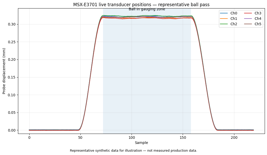
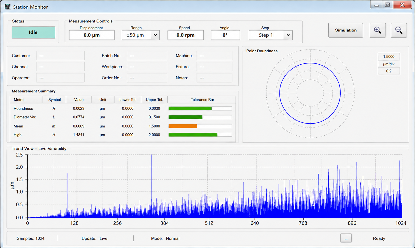
Install matplotlib and run sample_length_dashboard.py for a live chart of every probe, useful when aligning the ring and choosing the threshold value for Step 5.
More advanced applications can look like this :
Step 9: From samples to your production stack
The repository ships a complete, runnable sample suite for the MSX-E 3701/3700. Every sample reads the device address from the environment and is commented step by step.
| Sample | What it shows |
|---|---|
| sample_transducer_types.py | Supported transducer types and the selection_index every other sample needs |
| sample_transducer_database.py | Reading, adding and saving transducer definitions on the module |
| sample_minmax_measurement.py | Peak-hold gauging, the pattern behind this article |
| sample_length_polling.py | Timed position polling, tabular output |
| sample_length_continuous.py | Live display of every channel until Ctrl+C |
| sample_length_stream.py | sample_length_stream.py |
| sample_length_csv_logger.py | Data logger with CSV export straight into pandas, Excel or Grafana |
| sample_length_dashboard.py | Live matplotlib chart |
| sample_acquisition_finite.py | Finite capture of N sequences |
| sample_acquisition_continuous.py | Unbounded streaming into your own callback |
| sample_calibration.py | Guided calibration procedure, step by step |
| sample_connection_diagnostic.py | Line break and short-circuit detection per channel |
4. API Highlights
| Operation | What it does |
|---|---|
| get_number_of_types() / get_type_information(i) | Ask the module which transducers it supports: name, type, range, sensitivity, excitation frequency, impedance, and the selection_index used everywhere else. |
| minmax_start(…) / minmax_get_status() / minmax_stop() | Peak-hold gauging computed on the module. Optional self-stop when a watched channel crosses a threshold. Status returns min and max raw counts for all 16 channels. |
| auto_refresh_start() / auto_refresh_get_values() / auto_refresh_stop() | Continuous position polling over SOAP, for live display and setup. |
| acquire_finite(…) / acquire_continuous(callback, …) | Block capture and unbounded streaming over the dedicated data server, so control traffic and measurement data never compete. |
| Connection diagnosis | Primary and per-channel secondary connection and short-circuit tests, plus rearm_primary() recovery. |
| Calibration | calibration_start() / calibration_get_status() / calibration_next_step(), one guided run through primary feedback, 0 mm null point and displaced user position. |
| Transducer database | Add, delete and persist transducer definitions on the module itself, so the configuration travels with the hardware. |
| Offline by design | WSDLs bundled with the package; the client constructs with no internet access. |
5. Supported Configurations
| Version | Wandler | Transducer Type | Protection |
|---|---|---|---|
| MSX-E3701-HB-16 | 16 | Half-Bridge | IP 65 |
| MSX-E3701-HB-8 | 8 | Half-Bridge | IP 65 |
| MSX-E3701-LVDT-16 | 16 | LVDT | IP 65 |
| MSX-E3701-LVDT-8 | 8 | LVDT | IP 65 |
| MSX-E3701-K-8 | 8 | Knaebel | IP 65 |
| MSX-E3701-M-8 | 8 | Mahr-compatible | IP 65 |
| MSX-E3700-HB-16 | 16 | Half-Bridge | IP 40 |
| MSX-E3700-HB-8 | 8 | Half-Bridge | IP 40 |
| MSX-E3700-LVDT-16 | 16 | LVDT | IP 40 |
| MSX-E3700-LVDT-8 | 8 | LVDT | IP 40 |
- IP 65 – dust-tight, protected against water jets from any direction. Mounts at the machine.
- IP 40 – protected against foreign bodies > 1 mm. Enclosure mounting.
All versions operate from −40 °C to +85 °C. Knaebel and Mahr-compatible are offered on the MSX-E3701 only, in 8-channel form, if you already run those probes, the variant is decided for you.
6. What this changes on the line
- Every part measured, not a sample. Gauging happens in the flow, so the inspection rate is 100 % without a throughput penalty.
- Fewer components. Threshold self-stop removes the presence sensor; direct transducer inputs remove the conditioning rack.
- PLC cycle time preserved. The extremum is computed on the module; the PLC receives a result, not a signal to process.
- Range is a software decision. Change the probe, change the range, the same module and the same code cover the next gauging job.
- Traceability by design. Raw counts stay visible alongside millimetres, and calibration is the documented path between them.
- Feeds SPC directly. CSV output imports into Excel, pandas or Grafana as-is; continuous streaming feeds a time-series database or an ML pipeline for drift detection on the grinding process upstream.
7. Three ways to start, depending on where you sit:
You run a test bench or a validation programme?
Validate the technology on your own application before committing budget.
We provide a free loan unit with a working example tailored to your measurement task, support you in meeting your target performance, and provide the documentation required for your internal validation process.
Prove the concept first. Invest later.
You integrate condition monitoring for your customers?
Start with a documented and proven building block.
Request our reference architecture, including hardware, Python API, sample code and integration guidance. You benefit from predictable commissioning, clearly defined interfaces, and lifecycle commitments.
Reduce risk. Accelerate deployment.
You build the machine?
Integrate once and rely on it for the lifetime of your machine.
We support your design-in with product variants, dedicated part numbers and custom firmware whenever the standard offering does not fully match your requirements. Long-term availability and lifecycle commitments are provided in writing.
A measurement platform designed for long-term machine programmes.
8. Get Started
Download the Python API and samples from our GitHub repository:
- GitHub: https://github.com/ADDI-DATA/msxe-samples
- ConfigTools: https://www.addi-data.com/de/configtools
- Documentation: See README.md in the repository for full API reference
For technical support, please contact: [email protected]
Möchten Sie mehr erfahren?
If you want to learn more about the MSX-E3701, you can find additional information directly on the product page.
ADDI-DATA LÖSUNGEN
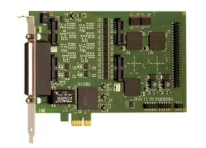
PC-Karten
• Für vielfältige Signaltypen
• Höchste Präzision
• Robust und störsicher
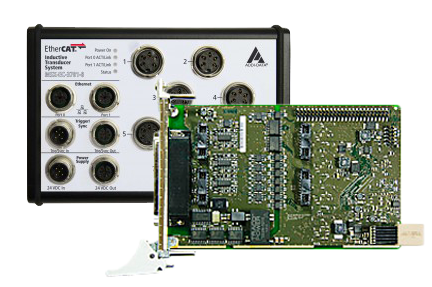
Echtzeit-Systeme
• EtherCAT und Profinet
• Systeme mit Linux inkl. Echtzeiterweiterung
• PC-Karten mit Treibern mit Echtzeit-Erweiterung RTX
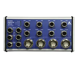
Ethernet-Systeme
• Direkter Sensoranschluss
• Integrierte Auswertung der erfassten Daten
• Für den Einsatz im Feld, bis IP 67
Datenlogger
• Langzeitdatenaufzeichnung vielfältiger Signaltypen
• Einrichtung der Messstelle ohne Programmierkenntnisse
• Visualisierung der Live-Daten
Lösungen nach Maß
Die bessere Lösung ist oft maßgeschneidert. Als Hersteller können wir unsere Lösungen
schnell und effizient an Ihren Bedürfnissen anpassen. Wir beraten Sie gerne um die optimale Lösung für Ihre Applikation zu finden und führen auch gerne die notwendige Anpassung für Sie durch.
Fragen Sie uns!